Research Article by Ernest HB, Vickers TW, Morrison SA, Buchalski MR, Boyce WM in PLOS ONE

Pumas in southern California live among a burgeoning human population of roughly 20 million people. To better understand how habitat loss, fragmentation, and human-caused puma mortality impact the puma population’s viability and genetic diversity, researchers have examined genetic status of pumas in coastal mountains within the Peninsular Ranges south of Los Angeles, in San Diego, Riverside, and Orange counties. These Santa Ana Mountains pumas show strong evidence of a genetic bottleneck and isolation from other populations in California. These and ecological findings provide a warning signal to wildlife managers and land use planners that mitigation efforts will be needed to stem further genetic and demographic decay in the Santa Ana Mountains puma population.

Abstract

Pumas (Puma concolor; also known as mountain lions and cougars) in southern California live among a burgeoning human population of roughly 20 million people. Yet little is known of the consequences of attendant habitat loss and fragmentation, and human-caused puma mortality to puma population viability and genetic diversity.

We examined genetic status of pumas in coastal mountains within the Peninsular Ranges south of Los Angeles, in San Diego, Riverside, and Orange counties. The Santa Ana Mountains are bounded by urbanization to the west, north, and east, and are separated from the eastern Peninsular Ranges to the southeast by a ten lane interstate highway (I-15). We analyzed DNA samples from 97 pumas sampled between 2001 and 2012. Genotypic data for forty-six microsatellite loci revealed that pumas sampled in the Santa Ana Mountains (n = 42) displayed lower genetic diversity than pumas from nearly every other region in California tested (n = 257), including those living in the Peninsular Ranges immediately to the east across I-15 (n = 55). Santa Ana Mountains pumas had high average pairwise relatedness, high individual internal relatedness, a low estimated effective population size, and strong evidence of a bottleneck and isolation from other populations in California.

These and ecological findings provide clear evidence that Santa Ana Mountains pumas have been experiencing genetic impacts related to barriers to gene flow, and are a warning signal to wildlife managers and land use planners that mitigation efforts will be needed to stem further genetic and demographic decay in the Santa Ana Mountains puma population.

Introduction

Genetic diversity, demography, and abundance — biological characteristics that influence population viability — can vary across a species’ distribution. Species that are generally perceived as wide-ranging and abundant are sometimes relegated to status as “least conservation concern”, in spite of indicators signaling concern and frequently, lack of data. Pumas (Puma concolor; also known as mountain lion, cougar, and in Florida, panther) epitomize this dilemma.

Although pumas in California have not been subjected to hunting since 1972, and were designated as a Specially Protected Mammal in 1990 [1], there is minimal active management and little scientifically validated data on statewide or regional population numbers. Pumas in southern California have one of the lowest annual survival rates among any population in North America, on par with rates seen in hunted populations (unpublished data). They are under increasing threats from habitat loss and fragmentation, and mortality from vehicle strikes, depredation permits, poaching, public safety kills, wildfire, and poisoning [2], [3]. Timely evaluation of potential threats to population viability is imperative in order to prioritize conservation activities to prevent collapse of some populations.

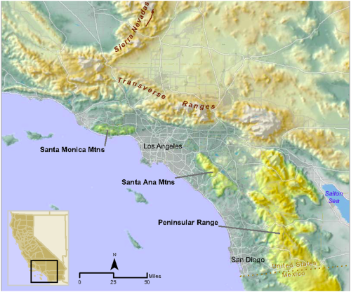
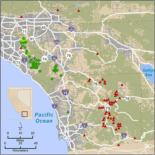
The human population of southern California is over 20 million [4] and expected to exceed 30 million by 2060 [5]. This increasing population will likely result in further loss, fragmentation, and degradation of natural habitats in the region. Habitat fragmentation south of greater Los Angeles has effectively turned the Santa Ana Mountain range in mostly Orange and Riverside counties into a ‘mega-fragment’ of habitat, surrounded to the west, north, and east by dense urban land uses. The only remaining montane and foothill habitat linkage connecting the Santa Ana Mountain range to other mountains of the Peninsular Range is a southeasterly swath of habitat bisected by a very heavily traveled 10-lane highway, Interstate 15 (I-15) (Figure 1).

FIGURE 1

Population viability of pumas in the Santa Ana Mountains (a geography henceforth referred to as distinct from the broader Peninsular Ranges to the east) has been of conservation concern for decades. Population monitoring and modeling in the 1980s highlighted that urbanization and highways were fragmenting puma habitat (e.g., [6], and that in turn motivated efforts to protect habitat connectivity in the region (e.g., [7], [8]). As part of a statewide assessment of puma genetic diversity and population structure, Ernest et al. [9] employed an 11-locus microsatellite panel and found that, for a limited sample size (n = 14) Santa Ana pumas had lower genetic diversity than other populations in California.

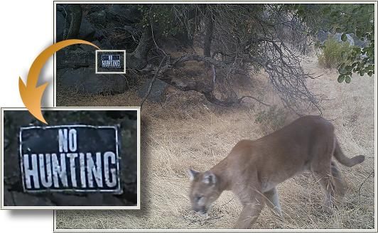
Since 2001, pumas in the region have been the subject of an ongoing study by the Karen C. Drayer Wildlife Health Center of the University of California, Davis (UCD) School of Veterinary Medicine. Visit the project’s website.

Telemetry data from 74 pumas in the UCD study has confirmed that minimal connectivity (only one GPS-collared puma over ten years was documented to transit successfully; unpublished data) exists between the Santa Ana Mountains and the eastern Peninsular Ranges across I-15, confirming that previous connectivity concerns were warranted.

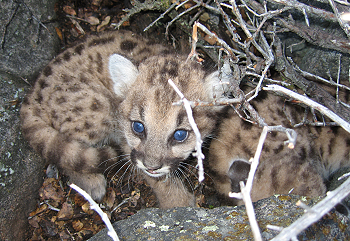
We conducted a detailed appraisal of the genetic diversity, relatedness, and population structure of southern California puma populations. Using 97 samples collected over 12 years as part of the UCD study, and a 46-locus microsatellite panel, we evaluated levels of genetic diversity, estimated effective population sizes and tested whether genetic data supported a hypothesis of recent bottleneck in the populations.

We assessed whether genetics reflected our telemetry observations of infrequent puma crossings of I-15 between the Santa Ana Mountains and the Peninsular Ranges to the east. Additionally we explored inter-population gene flow at multiple time scales by employing methods that reflect recent (a few generations) and more historical (tens or more generations).

Finally, we tested our hypothesis that the Santa Ana population had lower genetic diversity than those sampled from other regions in California.

Materials and Methods

Samples

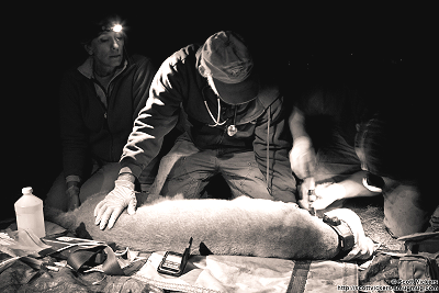
We obtained blood or tissue samples for analysis of nuclear DNA from pumas captured for telemetry studies, and from those found dead or killed by state authorities for livestock depredation or public safety in San Diego, Orange, Riverside, and San Bernardino counties of southern California (n = 97) during 2001-2012 (Figure 2). Pumas captured for telemetry were captured and sampled as detailed in [10]. Forty-two samples were collected to the west of I-15 in the Santa Ana Mountains, and 55 samples were collected in the Peninsular Ranges to the east of I-15. A small number of additional samples were collected from deceased animals in San Bernardino County just to the north of the Peninsular Range across Interstate Highway 10. For population genetic comparisons with pumas sampled elsewhere throughout California, a 257 sample subset of our statewide puma DNA data archive was employed (regions and sample sizes detailed in Table 1 and depicted in Figure 1 in [9]).

FIGURE 2

TABLE 1

Ethics Statement

Animal handling was carried out in strict accordance with the recommendations and approved Protocol 10950/PHS, Animal Welfare Assurance number A3433-01, with capture and sampling procedures approved by the Animal Care and Use Committee at the University of California, Davis (Protocol #17233), and Memoranda of Understanding and Scientific Collecting Permits from the California Department of Fish and Wildlife (CDFW). Permits and permissions for access to conserved lands at puma capture and sampling sites were obtained from CDFW, California Department of Parks and Recreation, The Nature Conservancy, United States (US) Fish and Wildlife Service, US Forest Service, US Bureau of Land Management, US Navy/Marine Corps, Orange County Parks Department, San Diego County Parks Department, San Diego State University, Vista Irrigation District, Rancho Mission Viejo/San Juan Company, Sweetwater Authority, California Department of Transportation (CalTrans), and the City of San Diego Water Department.

DNA Extraction and Microsatellite DNA Data Collection

Whole genomic DNA was extracted using the DNeasy Blood & Tissue Kit (QIAGEN, Valencia, CA, USA). Fifty microsatellite DNA primers were initially screened for this project. Forty-six loci that performed well in multiplex PCR (using the QIAGEN Multiplex PCR kit; QIAGEN) and conformed to expectations for Hardy-Weinberg and linkage equilibria were selected for ultimate analysis [11], [12], [13]. One sex-identification locus (Amelogenin) was used to confirm sex in samples from degraded puma carcasses [14].

PCR products were separated with an ABI PRISM 3730 DNA Analyzer (Applied Biosystems Inc., Foster City, CA, USA) with each capillary containing 1 µL of a 1:10 dilution of PCR product and deionized water, 0.05 µL GeneScan-500 LIZ Size Standard and 9.95 µL of HiDi formamide (both products Applied Biosystems Inc.) that was denatured at 95°C for 3 min. Products were visualized with STRand version 2.3.69 [15]. Negative controls (all reagents except DNA) and positive controls (well-characterized puma DNA) were included with each PCR run. Samples were run in PCR at each locus at least twice to assure accuracy of genotype reads and minimize risk of non-amplifying alleles. For >90% samples, loci that were heterozygous were run at least twice and homozygous loci were run at least three times.

Genetic Diversity

The number of alleles (Na), allelic richness (AR; incorporates correction for sample size), observed heterozygosity (Ho), expected heterozygosity (He), Shannon’s information index [16], and tests for deviations from Hardy-Weinberg equilibrium were calculated using software GenAlEx version 6.5 [17], [18]. Shannon’s information index provides an alternative method of quantifying genetic diversity and incorporates allele numbers and frequencies. Testing for deviations from expectations of linkage equilibrium was conducted using Genepop 4.2.1 [19], and we tested for the presence of null alleles using the program ML RELATE [20]. We assessed significance for calculations at alpha = 0.05 and used sequential Bonferroni corrections for multiple tests [21] in tests for Hardy-Weinberg and linkage equilibria.

The average probability of identity (PID) was calculated two ways using GenAlEx: 1) assuming random mating (PID_RM) without close relatives in a population [22], and 2) assuming that siblings with similar genotypes occur in a population (PID_SIBS) [23]. Probability of identity is the likelihood that two individuals will have the same genetic profile (genotype) for the DNA markers used. PID_SIBS is considered conservative since it probably conveys a higher likelihood; however, we recognized that siblings occurred in these populations.

Assessing Population Structure and Genetic Isolation

We used a Bayesian genetic clustering algorithm (STRUCTURE version 2.3.4 [24], [25]) to determine the likely number of population groups (K; genetic clusters) and to probabilistically group individuals without using the known geographic location of sample collection. We used the population admixture model with a flat prior and assumed that allele frequencies were correlated among populations, and ran 50,000 Markov chain Monte Carlo repetitions following a burnin period of 10,000 repetitions. First, an analysis including 354 statewide puma genotypes (97 from southern California and 257 from other regions) was run to estimate the probability of one through 10 genetic clusters (K), with each run iterated three times.

Second, given the output of the statewide run, we ran an analysis using only the 97 southern California puma genotypes to estimate the probability of one through five K, with each run iterated three times. Employing STRUCTURE HARVESTER [26] we averaged log probability of the data given K, log Pr(X|K), statistics across the multiple runs for each of the K estimates. In each case (statewide and southern California), we selected the K value of highest probability by identifying the set of values where the log Pr(X|K) value was maximized and subsequently selected the minimum value for K that did not sacrifice explanatory ability [27], [28], [29]. We defined membership to a cluster based upon the highest proportion of ancestry to each inferred cluster.

To further assess and visualize genetic relationships among regions and individuals, we performed principal coordinates analyses (PCoA) via covariance matrices with data standardization [30] using GenAlEx. This is a technique that allowed us to explore and plot the major patterns within the data sets.

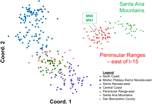
The PCoA process located major axes of variation within our multidimensional genotype data set. Because each successive axis explains proportionately less of the total genetic variation, the first two axes were used to reveal the major separation among individuals. Employing Genalex software, a pairwise, individual-by-individual genetic distance matrix was generated and then used to create the PCoA.

Wright’s F-statistic, F_ST, was calculated to appraise how genetic diversity was partitioned between populations. As implemented in GenAlEx, we used Nei’s [31] formula, with statistical testing options offered through 9999 random permutations and bootstraps.

Detecting Migrants

We used GENECLASS2 version 2.0.h [32] to identify first-generation migrants, i.e. individuals born in a population other than the one in which they were sampled. Genetic clusters identified during STRUCTURE analysis were treated as putative populations. GENECLASS2 provides different likelihood-based test statistics to identify migrant individuals, the efficacy of which depends on whether all potential source populations have been sampled. We first calculated the likelihood of finding a given individual in the population in which it was sampled, L_h, assuming all populations had not been sampled. We then calculated L_h/L_max, the ratio of L_h to the greatest likelihood among the populations [33], which has greater power when all potential source populations have been sampled. The critical value of the test statistic (L_h or L_h/L_max) was determined using the Bayesian approach of Rannala and Mountain [34] in combination with the resampling method of Paetkau et al. [33]; i.e., Monte Carlo simulations carried out on 10,000 individuals with the significance level set to 0.01.

Testing for Bottlenecks and Inferring Effective Population Size

We tested for evidence of recent population size reductions in Santa Ana Mountains and eastern Peninsular Range regions with one-tailed Wilcoxon sign-rank tests for heterozygote excess in the program BOTTLENECK version 1.2.02 [35]. The program evaluates whether the reduction of allele numbers occurred at a rate faster than reduction of heterozygosity, a characteristic of populations which have experienced a recent reduction of their effective population size (Ne) [35], [36]. This bottleneck genetic signature is detectable by this test for a finite time, estimated to be less than 4 times Ne generations [37]. These tests were performed using the two-phase (TPM, 70% step-wise mutation model and 30% IAM) model of microsatellite evolution and 10,000 iterations.

We then estimated contemporary Ne for each of the two regions based on gametic disequilibrium with sampling bias correction [38] using LDNE version 1.31 [39]. Ne is formally defined as the size of the ideal population that would experience the same amount of genetic drift as the observed population [40]. These analyses excluded alleles occurring at frequencies ≤0.05, and we used the jackknife method to determine 95% confidence intervals [38].

Relatedness Analyses: Pairwise Coefficient and Internal

Molecular kinship analysis was conducted using a number of software packages. Pairwise relatedness among individuals was evaluated using the algorithm of Lynch and Ritland [41], with reference allele frequencies calculated and relatedness values averaged within each southern California population, as implemented in GenAlEx. Partial molecular kinship reconstruction was conducted using a consensus of outputs from the GenAlEx pairwise relatedness calculator, ML Relate [20], CERVUS version 3.0.3 [42], and Colony version 2.0.3.1 [43], [44].

Individual genetic diversity (also called internal relatedness) was assessed using Rhh [45] as implemented in R statistical software [46]. This is a measure of genetic diversity within each individual (an estimate of parental relatedness [47], and we averaged over individuals for each of the two regions of southern California. Significance of differences between means was evaluated using t tests.

Results

Forty-two of the 46 loci that we employed were polymorphic in southern California and selected for the subsequent analyses. The average probabilities of identity with assumptions of either random mating (PID_RM) or mating among sibs (PID_SIBS) across the 42 loci for the eastern Peninsular Ranges were (PID_RM) 6.3×10^-22 and (PID_SIBS) 3.1×10^-10, and for the Santa Ana Mountains were (PID_RM) 2.8×10^-15 and (PID_SIBS) 1.1×10^-7 respectively. These very small values indicate that the panel of genetic markers provided very high resolution to distinguish individuals. For example, given this data the probability of seeing the same multi-locus genotype in more than one puma was less than one in nine million for Santa Ana Mountains pumas.

Genetic Diversity

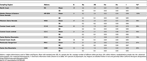
Measures of genetic variation including allelic diversity, heterozygosity, Shannon’s information index, and polymorphism, were lower for Santa Ana pumas than most of those tested from other regions of California (Table 1). Such low genetic diversity indicators were approached only by pumas in the Santa Monica Mountains (Ventura and Los Angeles Counties), a neighboring remnant puma population in the north Los Angeles basin (Figure 1).

Population Structure

Bayesian clustering analysis (STRUCTURE; Figure 3 of statewide puma genetic profiles (n = 354), including 97 from southern California, also support genetic distinctiveness of Santa Ana Mountains and eastern Peninsular Range pumas from other populations in the state. Three main genetic groups (A, B, and C) were evident in the analysis (Figure 3) The 97 pumas sampled in southern California (right-hand set of bars in Figure 3, with samples from Santa Ana and eastern Peninsular Range pumas labeled) predominantly cluster within genetic group C. The Santa Ana pumas assign very tightly to group C (0.996 average probability assignment), while pumas of the eastern Peninsular Ranges showed more variable assignment (0.93 average probability assignment), with 9 individuals (16%) having less than 0.90 assignment. Pumas sampled in the Central Coast of California (which included Santa Monica Mountains pumas) make up the central set of bands, and those individuals predominantly assign to the genetic group B. Pumas sampled in the other regions of California (North Coast Ranges, Modoc Plateau, western Sierra Nevada, and eastern Sierra Nevada) predominantly cluster with the genetic group A. Notably, there are individuals sampled in each geographic area which cluster with a genetic group that is not the dominant one in that area, suggesting dispersal events and/or genetic exchange that have occurred to varying degrees in each region.

FIGURE 3

A STRUCTURE analysis focused only on genetic data from the 97 southern California pumas indicated two distinct genetic groups (C-1 and C-2 shown in Figure 4). Pumas sampled in the eastern Peninsular Range region east of I-15 group primarily with C-2 and those of the Santa Ana Mountain region on the west side of I-15 group with C-1. An exception to the consistent genetic clustering was an adult male (M) puma (M86), that was captured in the Santa Ana Mountains but clustered with pumas from the eastern Peninsular Ranges (primarily genetic group C-2). Five other pumas captured in the Santa Ana Mountains had a 30-50% assignment to the C-2 group (M91, F92, M93, M97 and F102). Molecular kinship analysis showed that M86 and a female (F89) captured in the Santa Ana Mountains and assigned to the C-1 genetic group were the likely parents of three of these pumas (M91, F92, and M93) (results of relatedness and kinship analyses). M86 also was the likely parent of another puma in the group (M97), an offspring of another female (F61) that was sampled in Santa Ana Mountains and clustered with the C-1 genetic group. F102 was a <1 year old female killed by a vehicle in 2003 prior to collection of the majority of samples from adults in the Santa Ana Mountains.

FIGURE 4

Principal coordinates analysis of statewide puma genetic profiles (n = 354) (PCoA; Figure 5) allowed graphical examination of the first two major axes of multivariate genetic variation, and confirmed and added detail to the genetic distinctiveness of southern California pumas relative to others in California. The PCoA also reinforced the distinctiveness of pumas sampled in the Santa Ana Mountains from those sampled in the eastern Peninsular Ranges. Most pumas sampled in the Santa Ana Mountains align in a cloud of data points distinct from the eastern Peninsular Range pumas, and were the most genetically distant from all other pumas tested in California (Figure 5). The analysis also confirms the STRUCTURE findings that M86 who was sampled in the Santa Ana Mountains genetically aligns with the pumas sampled in the Peninsular Ranges, as does one of his offspring, M93 (see Figure 6 for additional detail). The PCoA position of data points for three pumas sampled in the San Bernardino Mountains north of Peninsular Ranges (pink diamonds in Figure 5) illustrates an intermediate genetic relationship between pumas from the rest of California and pumas sampled in the eastern Peninsular Ranges and Santa Ana Mountains, and suggests that they may represent transitional gene flow signature between southern California and regions to the north and east.

FIGURE 5

FIGURE 6

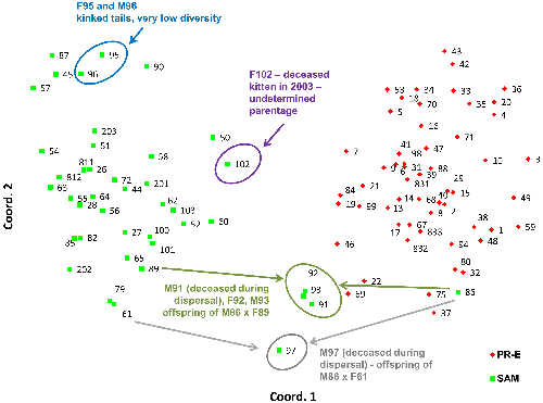
PCoA analysis of only the samples collected in the Santa Ana and Peninsular Ranges (Figure 6) confirms the findings from the STRUCTURE analysis indicating genetic distinctiveness of these two populations despite geographic proximity. Siblings M91, F92, and M93 (offspring of F89 and M86 according to our kinship reconstructions) as well as M97 (likely offspring of a female puma captured in the Santa Ana Mountains, F61, and M86, according to kinship reconstructions) are located graphically midway between their parents’ PCoA locations.

Genetic Isolation

Wright’s F_ST calculations (Table 2) indicate that Santa Ana Mountains pumas are the most isolated of those tested throughout California (p = 0.0001). Despite the short distance (as short as the distance across the I-15 Freeway) between the Santa Ana Mountains and the eastern Peninsular Range region, FST was surprisingly high (0.07) given the very close proximity of the two regions (separated only by an interstate highway). The Santa Monica Mountains pumas and Santa Ana Mountains pumas had the highest F_ST (0.27; lowest gene flow) of all pairwise comparisons in the state, demonstrating a high level of genetic isolation between these regions. The Santa Monica Mountains and Santa Ana Mountains are less than 100 km direct distance apart, through the center of Los Angeles. However the more likely distance for puma travel between these two mountain ranges, avoiding urban areas and maximizing upland habitat, would likely exceed 300 km (estimated using coarse measurements on Google Earth, Google, Inc.).

TABLE 2

Detection of Migrants

GENECLASS2 identified four individuals as first-generation migrants (P<0.01), four with the L_h method (pumas F75, M80, M86, and M99), and one with the L_h/L_max ratio (M86, which was detected using both likelihood methods). Pumas F75, M80, and M99 were all captured from the San Bernardino Mountains (Figure 2) at the northern extent of the study region, yet clustered with individuals from the Eastern Peninsular Range during STRUCTURE analysis. Their migrant designation may suggest immigration from populations north of Los Angeles and/or a distinct genetic population within the San Bernardino region. Puma M86 was captured in the Santa Ana Mountains, but assigned strongly to the eastern Peninsular Range genetic cluster, indicating a seemingly clear population of origin. This individual assignment is in accord with the clustering results from STRUCTURE (Figure 4).

Evidence of Genetic Bottlenecks

The Santa Ana Mountains population exhibited clear evidence of a population bottleneck (Table 3; Wilcoxon sign-rank test for heterozygote excess, and detection of a shift in the allele frequency distribution mode [36]; BOTTLENECK software). The eastern Peninsular Range mountain lions did not show a strong signature of a bottleneck.

TABLE 3

Effective Population Size

Effective population size (Ne) estimations using the linkage disequilibrium method (LDNe program) were 5.1 for the Santa Ana Mountains population and 24.3 for mountain lions in the eastern Peninsular Ranges. Statistical confidence intervals for both regions, given the genetic data, were tight (Table 3).

Relatedness: Pairwise Coefficient and Internal

The average pairwise coefficient of relatedness (r, Figure 7) was highest in Santa Ana Mountains pumas relative to all others tested in California (0.22; 95% confidence interval of 0.22-0.23), a level that approaches second order kinship relatedness (half-sibs, grantparent/grandchild, aunt-niece, etc). The value for the eastern Peninsular Ranges was 0.10 (confidence interval of 0.09-0.10), less than that of third order relatives (first cousins, great-grandparent/great grandchild). Other regions of California averaged similar or lower values to those of eastern Peninsular Ranges (Figure 7).

FIGURE 7

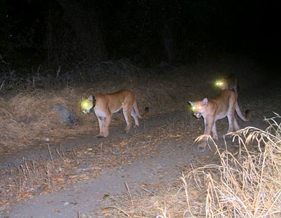
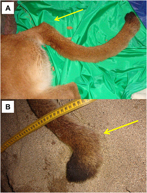
Among pumas sampled in the Santa Ana Mountains, the population average (0.14) for internal relatedness as implemented in rHH software was significantly higher (t test; p = 5.8×10^-6) than for those sampled in the eastern Peninsular Ranges (0.001). Of a group of six pumas which clustered near one another in PCoA (Figure 6), five have among the lowest individual genetic diversity measured in southern California (Puma ID [Internal Relatedness value: F45 [0.37], F51 [0.37], M87 [0.28], F90 [0.21], F95 [0.38], and M96 [0.33]). Notably, pumas F95 and M96 (highest internal relatedness) were observed with kinked tails at capture in the Santa Ana Mountains (Figure 8).

FIGURE 8

Discussion

Pumas of the Santa Ana Mountains are genetically depauperate, isolated, and display signs of a recent and significant bottleneck. In general, coastal California puma populations have less genetic diversity and less gene flow from other populations than those farther inland [9] (Table 1). This study showed that two coastal populations (Santa Ana Mountains and Santa Monica Mountains) had particularly low genetic variation and gene flow from other regions. Lack of gene flow is likely due in part to natural barriers to puma movement: geography and habitat (Pacific Ocean to the west; less hospitable desert habitat bounding certain regions, etc.). However, our data suggest that anthropogenic developments on the landscape are playing a large role in genetic decay in the Santa Ana Mountains puma population. As large solitary carnivores with sizable habitat requirements, pumas are extremely sensitive to habitat loss and fragmentation [48], [49].

The genetic bottleneck in the Santa Ana Mountains pumas is estimated at less than about 80 years, depending on definitions of effective population size (Ne) and puma generation time. Luikhart and Cornuet [37] state that the bottleneck signatures decay after “4 times Ne [here estimated to be 5.1] generations”. Logan and Sweanor [50] estimated generation time for their New Mexico population of pumas to be 29 months (2.4 years) for females. If an allowance of 2.4-4.0 years is made for generation times (unknown) in the Santa Ana Mountains population, the maximum estimated time since a bottleneck would be about 40-80 years. This was a period of tremendous urban development and multi-lane highway construction in southern California, particularly I-15 [51]. It is likely that the potential for connectivity between the Santa Ana Mountains and the Peninsular Range-East region will continue to be eroded by ongoing increases in traffic volumes on I-15, and conversion of unconserved lands along the I-15 corridor by development and agriculture [8], [48], [52].

An isolated population of pumas in the Santa Monica Mountains to the north of the Santa Ana Mountains also exhibit low values relative to other western North American populations (see Table 2 in [53]. Santa Monica pumas are isolated by urbanization of a megacity and busy wide freeways (Ventura county, including greater Los Angeles region [53]. Multiple instances of intraspecific predation, multiple consanguineous matings (father to daughter, etc.), and lack of successful dispersal highlight a suite of anthropogenic processes also occurring in the Santa Ana Mountains. Our collective findings of kinked tails and very low genetic diversity in Santa Ana pumas F95 and M96 may portend manifestations of genetic inbreeding depression similar to those seen in Florida panthers [54], [55]; however recognizing that kinked tails can have non-genetic etiologies.

Our analyses suggest that the Santa Ana Mountains puma population is highly challenged in terms of genetic connectivity and genetic diversity, a result hinted at in Ernest et al. [9] and now confirmed to be an ongoing negative process for this population. This compounds the demographic challenges of low survival rates and scant evidence of physical connectivity to the Peninsular Ranges east of I-15 (unpublished data). Beier [6] documented these same challenges during the 1990’s, and data from the ongoing UCD study suggest the trends have accelerated. Substantial habitat loss and fragmentation has occurred and is continuing to occur; Burdett et al. [10] estimated that by 2030, approximately 17% of puma habitat that was still available in 1970 in southern California will have been lost to development, and fragmentation will have rendered the remainder more hazardous for pumas to utilize. Riley et al [53] document a natural “genetic rescue” event: the 2009 immigration and subsequent breeding success of a single male to the Santa Monica Mountains. This introduction of new genetic material into the population was paramount to raising the critically low level of genetic diversity, as also exemplified by the human-mediated genetic augmentation of Florida Panthers with Texas puma stock [56].

These findings raise concerns about the current status of the Santa Ana Mountains puma population, and the longer-term outlook for pumas across southern California. In particular, they highlight the urgency to maintain — and enhance — what connectivity remains for pumas (and presumably numerous other species) across I-15. Despite warnings [6], [9] about potential serious impacts to the Santa Ana Mountains puma population if concerted conservation action was not taken, habitat connectivity to the Peninsular Ranges has continued to erode. We are hopeful that these new genetic results will motivate greater focus on connectivity conservation in this region. Indeed, the Santa Ana Mountains pumas may well serve as harbingers of potential consequences throughout California and the western United States if more attention is not paid to maintaining connectivity for wildlife as development progresses.

Acknowledgments

Samples, data, and expertise were provided by multiple people and agencies, including California Department of Fish and Wildlife (R. Botta, B Gonzales, M. Kenyon, P. Swift, S. Torres, D. Updike, and others), California State Parks, National Park Service, The Nature Conservancy, UC Davis Wildlife Health Center, UC Davis Veterinary Genetics Laboratory, and the US Geological Survey. We thank the following for their technical assistance: L. Dalbeck, T. Drazenovich, T. Gilliland, J. George, and M. Plancarte. GIS data management and project cartography was provided by B. Cohen and J. Sanchez. Field work assistance was provided by J. Bauer, C. Bell, P. Bryant, D. Dawn, M. Ehlbroch, D. Krucki, K. Logan, B. Martin, B. Millsap, M. Puzzo, D. Sforza, L. Sweanor, C. Wiley, E. York, and numerous volunteers. Thanks to E. Boydsen, K. Crooks, R. Fisher, and L. Lyren for assistance coordinating field projects and sample acquisition. We thank anonymous reviewers for their constructive comments.

Author Contributions

Conceived and designed the experiments: HBE TWV WMB. Performed the experiments: HBE TWV MRB WMB. Analyzed the data: HBE TWV MRB. Contributed reagents/materials/analysis tools: HBE TWV SAM WMB. Contributed to the writing of the manuscript: HBE TWV SAM MRB WMB.

References

1. Mansfield TM, Torres SG (1994) Trends in mountain lion depredation and public safety threats in California. Paper 33. Proceedings of the Sixteenth Vertebrate Pest Conference, Santa Clara, CA. Editors: WS Halverson and AC Crabb. University of California, Davis.

2. Riley SPD, Pollinger JP, Sauvajot RM, York EC, Bromley C, et al. (2006) FAST-TRACK: A southern California freeway is a physical and social barrier to gene flow in carnivores. Mol Ecol 15: 1733-1741.

3. Riley SPD, Bromley C, Poppenga RH, Uzal FA, White L, et al. (2007) Anticoagulant exposure and notoedric mange in Bobcats and Mountain Lions in urban Southern California. J Wildl Manage 71: 1874-1884.

4. U.S. Census Bureau (2012) 2010 Census of Population and Housing, Summary Population and Housing Characteristics, CPH-1-6, California, U.S. Government Printing Office, Washington, DC.

5. California Department of Finance (2013) New Population Projections: California to surpass 50 million in 2049. Press release. Available: http://www.dof.ca.gov/research/demographic/reports/projections/p-1/documents/Projections_Press_Release_2010-2060.pdf Accessed 2 December 2013.

6. Beier P (1995) Dispersal of juvenile cougars in fragmented habitat. J Wildl Manage 59: 228-237.

7. Luke C, Penrod K, Cabanero CR, Beier P, Spencer W, et al. (2004) A Linkage Design for the Santa Ana-Palomar Mountains Connection. Unpublished report. San Diego State University, Field Station Programs and South Coast Wildlands. Available at: http://www.scwildlands.org/reports/SCML_SantaAna_Palomar.pdf.

8. Morrison SA, Boyce WM (2009) Conserving connectivity: Some lessons from mountain lions in southern California. Conserv Biol 23: 275-285.

9. Ernest HB, Boyce WM, Bleich VC, May B, Stiver SJ, et al. (2003) Genetic structure of mountain lion (Puma concolor) populations in California. Conserv Genet 4: 353-366.

10. Burdett CL, Crooks KR, Theobald DM, Wilson KR, Boydston EE, et al. (2010) Interfacing models of wildlife habitat and human development to predict the future distribution of puma habitat. Ecosphere 1: 1.

11. Ernest HB, Penedo MCT, May BP, Syvanen M, Boyce WM (2000) Molecular tracking of mountain lions in the Yosemite Valley region in California: genetic analysis using microsatellites and faecal DNA. Mol Ecol 9: 433-441.

12. Kurushima JD, Collins JA, Well JA, Ernest HB (2006) Development of 21 microsatellite loci for puma (Puma concolor) ecology and forensics. Mol Ecol Notes 6: 1260-1262.

13. Menotti-Raymond M, David VA, Lyons LA, Schaffer AA, Tomlin JF, et al. (1999) A genetic linkage map of Microsatellites of the domestic cat (Felis catus). Genomics 57: 9-23.

14. Pilgrim KL, Mckelvey KS, Riddle AE, Schwartz MK (2005) Felid sex identification based on noninvasive genetic samples. Mol Ecol Notes 5: 60-61. doi: 10.1111/j.1471-8286.2004.00831.x 15. Toonen RJ, Hughes S (2001) Increased throughput for fragment analysis on an ABI Prism 377 automated sequencer using a membrane comb and STRAND software. BioTechniques 31: 1320-1324.

16. Sherwin WB, Jabot F, Rush R, Rossetto M (2006) Measurement of biological information with applications from genes to landscapes. Mol Ecol 15: 2857-2869.

17. Peakall R, Smouse PE (2006) GenAlEx 6: genetic analysis in Excel. Population genetic software for teaching and research. Mol Ecol Notes 6, 288-295.

18. Peakall R, Smouse PE (2012) GenAlEx 6.5: genetic analysis in Excel. Population genetic software for teaching and research – an update. Bioinformatics 28: 2537-2539.

19. Rousset F (2008) genepop’007: a complete re-implementation of the genepop software for Windows and Linux. Mol Ecol Resour 8: 1755-0998.

20. Kalinowski ST, Wagner AP, Taper ML (2006) ML-RELATE: a computer program for maximum likelihood estimation of relatedness and relationship. Mol Ecol 6: 576-579.

21. Rice WR 1989. Analysing tables of statistical tests. Evolution 43: 223-5.

22. Taberlet P, Luikart G (1999) Non-invasive genetic sampling and individual identification. Biol J Linn Soc 68: 41-55.

23. Waits LP, Luikart G, Taberlet P (2001) Estimating the probability of identity among genotypes in natural populations: cautions and guidelines. Mol Ecol 10: 249-56.

24. Pritchard JK, Stephens M, Donnelly P (2000) Inference of population structure using multilocus genotype data. G3 155: 945-959.

25. Hubisz MJ, Falush D, Stephens M, Pritchard J (2009) Inferring weak population structure with the assistance of sample group information. Mol Ecol Resour 9: 1322-1332.

26. Earl DA, vonHoldt BM (2012) STRUCTURE HARVESTER: a website and program for visualizing STRUCTURE output and implementing the Evanno method. Conserv Genet Resour 4: 359-361.

27. Pritchard JK, Wen W (2002) Documentation for structure version 2.3.4. As viewed June 1 2013: http://pritch.bsd.uchicago.edu.

28. Evanno G, Regnaut S, Goudet J (2005) Detecting the number of clusters of individuals using the software STRUCTURE: a simulation study. Mol Ecol 14: 2611-2620.

29. Waples RS, Gaggiotti O (2006) What is a population? An empirical evaluation of some genetic methods for identifying the number of gene pools and their degree of connectivity. Mol Ecol 15, 1419-1439.

30. Orloci L (1978) Multivariate analysis in vegetation research. 2nd ed. Dr W. Junk. The Hague. 451 p.

31. Nei M (1977) F-statistics and analysis of gene diversity in subdivided populations. Ann Hum Genet 41: 225-233.

32. Piry S, Alapetite A, Cornuet JM, Paetkau D, Baudouin L (2004) GENECLASS2: A software for genetic assignment and first-generation migrant detection. J Hered 95: 536-539.

33. Paetkau D, Slade R, Burdens M, Estoup A (2004) Genetic assignment methods for the direct, real-time estimation of migration rate: a simulation-based exploration of accuracy and power. Mol Ecol 13: 55-65.

34. Rannala B, Mountain JL (1997) Detecting immigration by using multilocus genotypes. Proc Natl Acad Sci USA 94: 9197-9201.

35. Cornuet JM, Luikart G (1997) Description and power analysis of two tests for detecting recent population bottlenecks from allele frequency data. G3 144: 2001-2014.

36. Luikart G, Allendorf FW, Cornuet JM, Sherwin WB (1998) Distortion of allele frequency distributions provides a test for recent population bottlenecks. J Hered 89: 238-247.

37. Luikart G, Cornuet JM (1998) Empirical evaluation of a test for identifying recently bottlenecked populations from allele frequency data. Conserv Biol 12: 228-237.

38. Waples RS (2006) A bias correction for estimates of effective population size based on linkage disequilibrium at unlinked gene loci. Conserv Genet 7: 167-184.

39. Waples RS, Do C (2008) LDNE: a program for estimating effective population size from data on linkage disequilibrium. Mol Ecol Resour 8: 753-756.

40. Wright S (1969) Evolution and the Genetics of Population. Vol 2. The Theory of Gene Frequencies. University of Chicago Press.

41. Lynch M, Ritland K (1999) Estimation of pairwise relatedness with molecular markers. G3 152: 1753-1766.

42. Kalinowski ST, Taper ML, Marshall TC (2007) Revising how the computer program CERVUS accommodates genotyping error increases success in paternity assignment. Mol Ecol 16: 1099-1006.

43. Jones OR, Wang J (2010) COLONY: a program for parentage and sibship inference from multilocus genotype data. Mol Ecol Resour 10: 551-555.

44. Wang J (2012) Computationally efficient sibship and parentage assignment from multilocus marker data. G3 191: 183-194.

45. Alho JS, Välimäki K, Merilä J (2010) Rhh: an R extension for estimating Multilocus heterozygosity and heterozygosity-heterozygosity correlation. Mol Ecol Resour 10: 720-72.

46. R Development Core Team (2011) R: A language and environment for statistical computing. R Foundation for Statistical Computing, Vienna, Austria.

47. Amos W, Worthington Wilmer J, Fullard K, Burg TM, Croxall JP (2001) The influence of parental relatedness on reproductive success. Proc R Soc Lond B Biol Sci 268: 2021-2027.

48. Beier P (1993) Determining Minimum Habitat Areas and Habitat Corridors for Cougars. Conserv Biol 7: 94-108.

49. Crooks KR (2002) Relative Sensitivities of Mammalian Carnivores to Habitat Fragmentation. Conserv Biol 16: 488-502.

50. Logan K and Sweanor L (2001) Desert Puma: Evolutionary Ecology And Conservation Of An Enduring Carnivore. Island Press. 464.

51. Barbour E (2002) Metropolitan growth planning in California, 1900-2000. Public Policy Institute of California. San Francisco, California. 246.

52. Beier P (1996) Metapopulation modeling, tenacious tracking, and cougar conservation. In McCullough DR, editor, Metapopulations and wildlife management. Washington DC: Island Press. 293-323.

53. Riley SPD, Serieys LEK, Pollinger J, Sikich J, Dalbeck L, et al. Individual behaviors dominate the dynamics of an urban mountain lion population isolated by roads. Curr Biol 24: 1989-1994.

54. Roelke ME, Martenson JS, O’Brien SJ (1993) The consequences of demographic reduction in the endangered Florida panther. Curr Biol 3: 340-350.

55. Culver M, Hedrick PW, Murphy K, O’Brien S Hornocker MG (2008) Estimation of the bottleneck size in Florida panthers. Anim Conserv 11: 104-110.

56. Johnson WE, Onorato DP, Roelke ME, Land ED, Cunningham M, et al. (2010). Genetic restoration of the Florida panther. Science 329, 1641-1645.

This article is available for free thanks to PLOS ONE’s open access policy.